Orbital Mechanics Simulator | Neutron STEM Lab

Interactive workspace initializes in your browser. Engineering method, assumptions, validation, and references are available below.

Engineering reference

Orbit Simulator: theory, method, and sources

This aerospace & rocket science workspace publishes 10 governing equations, 5 stated assumptions, 5 documented boundaries, 2 worked examples, 3 validation cases, and 4 sources so the numbers it returns can be checked rather than taken on trust.

Calculations run locallyContent reviewed September 10, 2026Calculation & source methodology

How this tool works

Propagate spacecraft trajectories with a bounded fourth-order Runge–Kutta integrator using ideal two-body gravity and an optional first-order J2 acceleration term.

Initialize the spacecraft from classical orbital elements or Cartesian position/velocity, then convert between representations and inspect the resulting osculating elements.

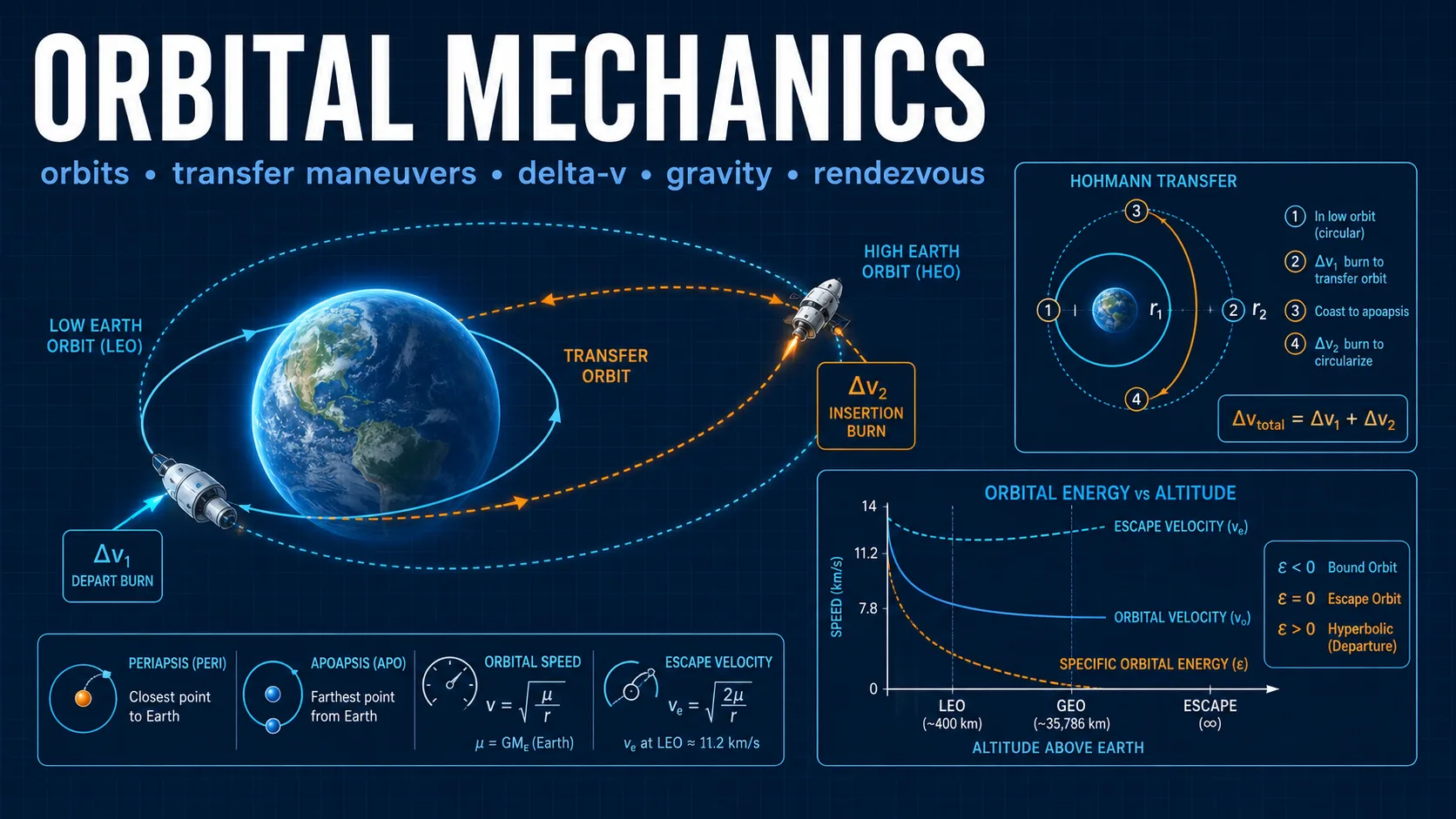
Schedule up to 20 impulsive maneuvers in the local radial/transverse/normal frame. Load both burns of a circular-orbit Hohmann transfer, or explore an ideal heliocentric transfer between any two of the eight planets. Animate the path and export trajectory samples as CSV.

Engineering theory

A state vector and orbital elements describe the same two-body orbit

Cartesian position and velocity are convenient for numerical propagation and maneuvers, while classical elements describe the conic geometry and its orientation. The simulator converts both representations so a user can inspect how a burn changes semi-major axis, eccentricity, inclination, node, periapsis orientation, and anomaly.

Circular and equatorial orbits contain geometric singularities in the classical element definitions. In those cases the simulator uses stable fallback angle conventions rather than implying that an undefined node or periapsis direction has unique physical meaning.

Impulsive burns are evaluated in the local RTN frame

The radial axis points away from the central body, the transverse axis lies in the instantaneous orbital plane in the direction of motion, and the normal axis is parallel to orbital angular momentum. This makes prograde/retrograde, radial, and plane-changing components easier to reason about than inertial XYZ velocity changes.

A real thruster burns over finite time and changes spacecraft mass. The instantaneous RTN impulse is therefore a mission-design approximation, not a propulsion execution model.

Numerical propagation should be checked for convergence

The simulator uses RK4 with a user-selected maximum step, reduced near fast motion and at maneuver events. Plotted output is decimated separately from integration so long runs do not silently enlarge the physics step. If the trajectory changes materially when the time step is reduced, the coarse result is not numerically converged. The two-body mode reports specific-mechanical-energy drift as one useful numerical diagnostic.

J2 changes the conservative potential, so the simple two-body energy diagnostic is intentionally disabled when J2 propagation is active.

Inputs and outputs explained

Inputs

Central body: Preset Sun/planet/moon or custom gravitational parameter, radius, and optional J2 coefficient.
Classical elementskm, degrees: Semi-major axis, eccentricity, inclination, RAAN, argument of periapsis, and true anomaly.
Cartesian state vectorkm, km/s: Inertial position and velocity components relative to the central body.
Propagation durationhours: Requested trajectory duration.
Integration steps: Maximum RK4 step. Local orbital timescales and exact maneuver times can shorten it; displayed samples are bounded independently.
RTN burnm/s: Up to 20 optional radial, transverse, and normal impulsive velocity changes at selected simulation times. Equal-time burns execute in list order.

Outputs

Trajectory: Time history of inertial position and velocity plus derived altitude and speed.
Osculating elements: Classical elements derived from the propagated final Cartesian state.
Altitude envelopekm: Minimum and maximum radius above the modeled body surface.
Peak speedkm/s: Maximum propagated inertial speed.
Energy drift: Relative change in two-body specific mechanical energy for runs without J2 or an impulse.
Hohmann preview: First/second burn, total Δv, and half-ellipse transfer time for circular-to-circular transfer planning.

Calculators and topics covered

orbital mechanics
orbit simulator
astrodynamics
spacecraft trajectory
Hohmann transfer
maneuver
state vector
orbital elements
free orbital mechanics simulator
online orbit simulator
spacecraft orbit propagation
classical orbital elements
impulsive burn
RTN burn

Core equations

\ddot{r} = \frac{- \mu r}{r^{3}}

v^{2} = \mu \left(\frac{2}{r} \frac{- 1}{a}\right)

p = a \left(1 - e^{2}\right)

r = \frac{p}{1 + e\; \cos \nu }

T = 2 \pi \sqrt{\frac{a^{3}}{\mu }}

\Delta v_{\mathrm{RTN}} = \Delta vR\; \hat{r} + \Delta vT\; \hat{t} + \Delta vN\; \hat{n}

aJ_{2} \propto \frac{\left(\frac{3}{2}\right) J_{2}\; \mu R^{2}}{r^{5}}

t_{\mathrm{transfer}} = \pi \sqrt{\frac{a_{\mathrm{transfer}}^{3}}{\mu Sun}}

\varphi _{\mathrm{departure}} = \pi - n_{\mathrm{arrival}}\; t_{\mathrm{transfer}}

\Delta v_{\mathrm{stage}} = I_{\mathrm{sp}}\; g_{0}\; \ln \left(\frac{m_{\mathrm{initial}}}{m_{\mathrm{final}}}\right)

Worked examples

400 km Earth orbit

Start near a 400 km circular Earth orbit with a 51.6° inclination and propagate slightly more than one revolution.

Inputs

a ≈ 6778.137 km
e = 0
i = 51.6°
J2 off

Result: The trajectory closes after about 92.6 minutes and the altitude remains approximately constant in the ideal two-body model.

Interpretation: Reducing the integration step should make the specific-energy drift approach zero.

LEO to GEO Hohmann transfer

Start from a circular 400 km Earth orbit and target a 35,786 km circular altitude.

Result: Loading the transfer scenario starts from a circular orbit, applies the first burn at departure and the circularization burn at the opposite apsis, then coasts to show the final orbit.

Interpretation: Both timed burns appear in the editable maneuver list and the execution table. Disable either burn to see why both are needed.

Common mistakes

Using an ideal phase angle as a launch date

The planet planner starts at an assumed alignment and uses circular mean orbits.

Better approach: Use its roughly 259-day Earth–Mars transfer to learn the geometry; use ephemerides and a targeting solver for actual launch dates.

Entering altitude as semi-major axis

Classical semi-major axis is measured from the central-body center, not from its surface.

Better approach: For a circular Earth orbit at altitude h, use a = R_Earth + h.

Treating RTN and XYZ as the same frame

A transverse burn is defined relative to the instantaneous orbit, not the inertial X or Y axis.

Better approach: Use the RTN labels when reasoning about prograde/retrograde, radial, or normal maneuver components.

Using a large step because the path still looks smooth

A smooth rendered polyline can hide integration error.

Better approach: Repeat the run with a smaller step and compare the final state or energy-drift diagnostic.

Reading a J2 run as a complete perturbation model

J2 is only one perturbation and does not include drag, third bodies, radiation pressure, tesseral harmonics, or real ephemerides.

Better approach: Use dedicated astrodynamics software for operational orbit prediction.

Method and assumptions

Convert the selected initial representation into an inertial Cartesian state.

Integrate r¨ = a(r) with bounded-step RK4. If enabled, add the selected body J2 acceleration.

At the requested maneuver time, construct the local RTN basis from position and angular momentum and apply the instantaneous Δv.

Derive final osculating elements, trajectory extrema, impact state, and numerical diagnostics from the propagated history.

Assumptions

The propagation frame is central-body-centered and inertial; the central body itself is fixed at the origin.
The base model uses point-mass two-body gravity. Optional J2 adds only the standard first-order oblateness acceleration for the selected body constant.
Impulsive burns change velocity instantaneously in the local RTN frame and do not model finite thrust, propellant depletion, attitude dynamics, or execution uncertainty.
Hohmann guidance assumes circular coplanar orbits. Planet transfers use fixed mean heliocentric radii and patched-conic parking-orbit departure/capture estimates; they do not find calendar launch windows.
Preset body constants are fixed educational reference values rather than time-dependent ephemerides.

Limitations and design boundaries

This is an educational and preliminary mission-design simulator, not an operational flight-dynamics, navigation, conjunction-assessment, or maneuver-certification tool.
The propagator does not include atmospheric drag, third-body gravity, solar radiation pressure, finite burns, low-thrust propagation, Lambert targeting, real ephemerides, covariance propagation, collision avoidance, or n-body integration.
The canvas uses an orthographic 3D projection for visualization. Apparent screen distances are not a perspective camera measurement.
Very long or stiff trajectories require dedicated astrodynamics software and validated numerical methods. Runs stop at a bounded integration work limit and show partial-run warnings.
The optional rocket panel is an ideal staging and launch-budget estimate. Exploring its chosen parking orbit assumes successful insertion; powered atmospheric ascent, gravity turns, drag and staging trajectories are not simulated.

Validation cases

These checks document how representative calculations are cross-checked against analytic or reference results.

Validation policy

Circular Earth orbit period

Analytic cross-check

Method: Convert a = Earth radius + 400 km, e = 0 to Cartesian state and evaluate T = 2π√(a³/μ).
Expected: Approximately 92.56 minutes.
Tolerance: Within numerical rounding of the fixed Earth μ and radius used by the tool.

Elements ↔ state round trip

Verified result

Method: Convert a non-singular elliptical orbit to Cartesian state and back to classical elements.
Expected: Semi-major axis, eccentricity, inclination, RAAN, argument of periapsis, and true anomaly return within floating-point tolerance.

Two-body energy conservation